tf <- dfm |>
tidytext::tidy() |>
dplyr::left_join(
dplyr::select(tbl, doc_id, section),
by = dplyr::join_by(document == doc_id)
) |>
dplyr::summarise(tf = sum(count), .by = term) |>
dplyr::pull(tf, term)
# modified from https://www.r-bloggers.com/2019/08/correspondence-analysis-visualization-using-ggplot/
make_ca_plot_df <- function(ca.plot.obj, row.lab = "Rows", col.lab = "Columns") {
tibble::tibble(
Label = c(
rownames(ca.plot.obj$rows),
rownames(ca.plot.obj$cols)
),
Dim1 = c(
ca.plot.obj$rows[, 1],
ca.plot.obj$cols[, 1]
),
Dim2 = c(
ca.plot.obj$rows[, 2],
ca.plot.obj$cols[, 2]
),
Variable = c(
rep(row.lab, nrow(ca.plot.obj$rows)),
rep(col.lab, nrow(ca.plot.obj$cols))
)
)
}
dat <- dat |>
make_ca_plot_df(row.lab = "Construction", col.lab = "Medium") |>
dplyr::mutate(
Size = dplyr::if_else(Variable == "Construction", mean(tf), tf[Label])
)
# 非ASCII文字のラベルに対してwarningを出さないようにする
suppressWarnings({
ca_sum <- summary(ca_fit)
dim_var_percs <- ca_sum$scree[, "values2"]
})
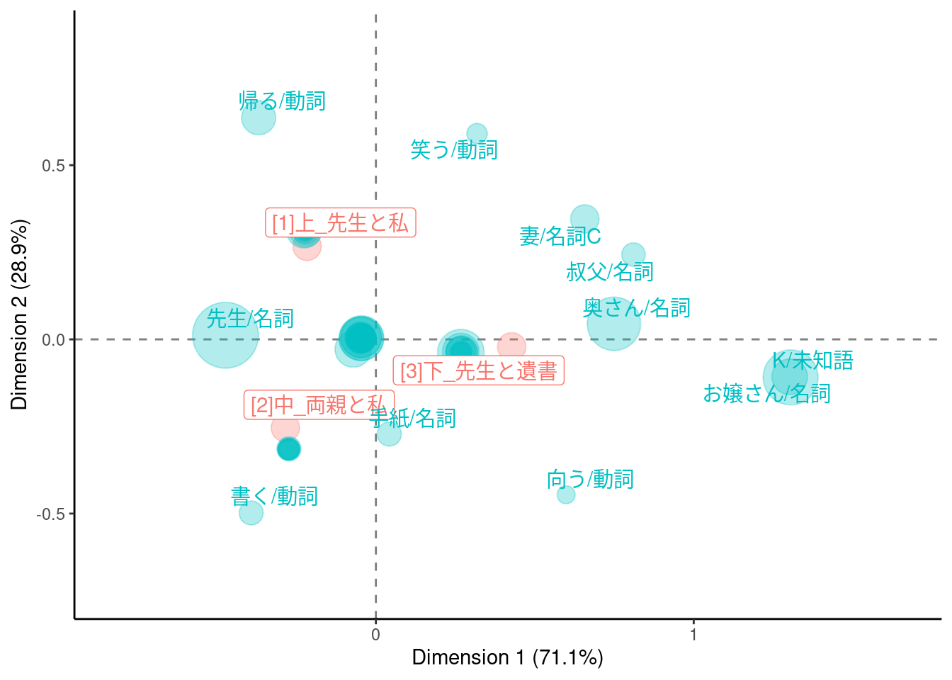
dat |>
ggplot(aes(x = Dim1, y = Dim2, col = Variable, label = Label)) +
geom_vline(xintercept = 0, lty = "dashed", alpha = .5) +
geom_hline(yintercept = 0, lty = "dashed", alpha = .5) +
geom_jitter(aes(size = Size), alpha = .3, show.legend = FALSE) +
ggrepel::geom_label_repel(
data = \(x) dplyr::filter(x, Variable == "Construction"),
show.legend = FALSE
) +
ggrepel::geom_text_repel(
data = \(x) dplyr::filter(x, Variable == "Medium", sqrt(Dim1^2 + Dim2^2) > 0.25),
show.legend = FALSE
) +
scale_x_continuous(
limits = range(dat$Dim1) +
c(diff(range(dat$Dim1)) * -0.2, diff(range(dat$Dim1)) * 0.2)
) +
scale_y_continuous(
limits = range(dat$Dim2) +
c(diff(range(dat$Dim2)) * -0.2, diff(range(dat$Dim2)) * 0.2)
) +
scale_size_area(max_size = 16) +
labs(
x = paste0("Dimension 1 (", signif(dim_var_percs[1], 3), "%)"),
y = paste0("Dimension 2 (", signif(dim_var_percs[2], 3), "%)")
) +
theme_classic()
#> Warning: ggrepel: 24 unlabeled data points (too many overlaps). Consider
#> increasing max.overlaps