suppressPackageStartupMessages({
  library(ggplot2)
  library(duckdb)
  library(arules)
  library(arulesViz)
  library(ca)
})
drv <- duckdb::duckdb()
con <- duckdb::dbConnect(drv, dbdir = "tutorial_jp/kokoro.duckdb", read_only = TRUE)

tbl <-
  readxl::read_xls("tutorial_jp/kokoro.xls",
    col_names = c("text", "section", "chapter", "label"),
    skip = 1
  ) |>
  dplyr::mutate(
    doc_id = factor(dplyr::row_number()),
    dplyr::across(where(is.character), ~ audubon::strj_normalize(.))
  ) |>
  dplyr::filter(!gibasa::is_blank(text)) |>
dplyr::relocate(doc_id, text, section, label, chapter)Appendix C — 抽出語メニュー2
C.1 関連語検索(A.5.6)
C.1.1 関連語のリスト
「確率差」や「確率比」については、いちおう計算はできた気がしますが、あっているのかよくわからないです。また、このやり方はそれなりの数の共起について計算をしなければならず、共起行列が大きくなると大変そうなため、あまりおすすめしません。
dfm <-
  dplyr::tbl(con, "tokens") |>
  dplyr::filter(
    section == "[1]上_先生と私",
    pos %in% c(
      "名詞", # "名詞B", "名詞C",
      "地名", "人名", "組織名", "固有名詞",
      "動詞", "未知語", "タグ"
    )
  ) |>
  dplyr::mutate(
    token = dplyr::if_else(is.na(original), token, original),
    token = paste(token, pos, sep = "/")
  ) |>
  dplyr::count(doc_id, token) |>
  dplyr::collect() |>
  tidytext::cast_dfm(doc_id, token, n) |>
  quanteda::dfm_weight(scheme = "boolean")

dat <- dfm |>
  quanteda::fcm() |>
  tidytext::tidy() |>
  dplyr::rename(target = document, co_occur = count) |>
  rlang::as_function(~ {
    col_sums <- quanteda::colSums(dfm)
    dplyr::reframe(.,
      term = term,
      target_occur = col_sums[target],
      term_occur = col_sums[term],
      co_occur = co_occur,
      .by = target
    )
  })() |>
  dplyr::mutate(
    p_x = target_occur / quanteda::ndoc(dfm),
    p_y = term_occur / quanteda::ndoc(dfm),
    p_xy = (co_occur / quanteda::ndoc(dfm)) / p_x,
    differential = p_xy - p_y, # 確率差
    lift = p_xy / p_y, # 確率比(リフト),
    jaccard = co_occur / (target_occur + term_occur - co_occur),
    dice = 2 * co_occur / (target_occur + term_occur)
  ) |>
  dplyr::select(target, term, differential, lift, jaccard, dice)

dat
#> # A tibble: 26,820 × 6
#>    target    term            differential  lift jaccard    dice
#>    <chr>     <chr>                  <dbl> <dbl>   <dbl>   <dbl>
#>  1 先生/名詞 知り合い/名詞       0.00790  2.10  0.0151  0.0297
#>  2 先生/名詞 海水浴/名詞         0.000176 1.05  0.00376 0.00749
#>  3 先生/名詞 帰る/動詞           0.0150   1.20  0.0848  0.156
#>  4 先生/名詞 断る/動詞           0.000529 1.05  0.0112  0.0221
#>  5 先生/名詞 一人/タグ           0.0129   1.40  0.0443  0.0848
#>  6 先生/名詞 大分/地名          -0.00145  0.839 0.00746 0.0148
#>  7 先生/名詞 鎌倉/地名           0.00430  1.40  0.0150  0.0295
#>  8 先生/名詞 探す/動詞          -0.00162  0.699 0.00375 0.00746
#>  9 先生/名詞 建てる/動詞         0.000176 1.05  0.00376 0.00749
#> 10 先生/名詞 通り抜ける/動詞    -0.00342  0.525 0.00373 0.00743
#> # ℹ 26,810 more rows
C.1.2 共起ネットワーク
「先生/名詞」と関連の強そうな語の共起を図示した例です。
「先生/名詞」と共起している語のうち、出現回数が上位20位以内である語がtargetである共起を抽出したうえで、それらのなかからJaccard係数が大きい順に75個だけ残しています。「先生/名詞」という語そのものは図に含めていません。
dat |>
  dplyr::inner_join(
    dplyr::filter(dat, target == "先生/名詞") |> dplyr::select(term),
    by = dplyr::join_by(target == term)
  ) |>
  dplyr::filter(target %in% names(quanteda::topfeatures(dfm, 20))) |>
  dplyr::slice_max(jaccard, n = 75) |>
  tidygraph::as_tbl_graph(directed = FALSE) |>
  tidygraph::to_minimum_spanning_tree() |>
  purrr::pluck("mst") |>
  dplyr::mutate(
    community = factor(tidygraph::group_leading_eigen())
  ) |>
  ggraph::ggraph(layout = "fr") +
  ggraph::geom_edge_link(aes(width = sqrt(lift), alpha = jaccard)) +
  ggraph::geom_node_point(aes(colour = community), show.legend = FALSE) +
  ggraph::geom_node_text(aes(label = name, colour = community), repel = TRUE, show.legend = FALSE) +
  ggraph::theme_graph()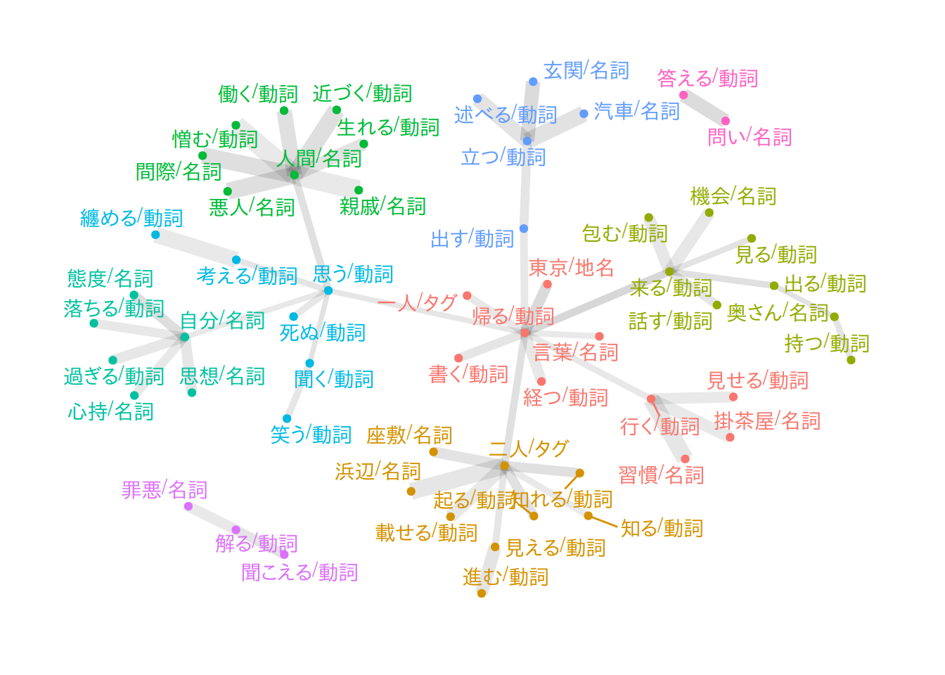
C.1.3 アソシエーション分析🍳
英語だとこのメニューの名前は「Word Association」となっているので、ふつうにアソシエーション分析すればいいと思いました。
arulesのtransactionsオブジェクトをつくるには、quantedaのfcmオブジェクトから変換すればOKです(arulesをアタッチしている必要があります)。
library(arules)
library(arulesViz)

dat <-
  dplyr::tbl(con, "tokens") |>
  dplyr::filter(
    pos %in% c(
      "名詞", # "名詞B", "名詞C",
      "地名", "人名", "組織名", "固有名詞",
      "動詞", "未知語", "タグ"
    )
  ) |>
  dplyr::mutate(
    token = dplyr::if_else(is.na(original), token, original),
    token = paste(token, pos, sep = "/")
  ) |>
  dplyr::count(doc_id, token) |>
  dplyr::collect() |>
  tidytext::cast_dfm(doc_id, token, n) |>
  quanteda::dfm_weight(scheme = "boolean") |>
  quanteda::fcm() |>
  as("nMatrix") |>
as("transactions")arules::apriori()でアソシエーションルールを抽出します。
rules <-
  arules::apriori(
    dat,
    parameter = list(
      support = 0.075,
      confidence = 0.8,
      minlen = 2,
      maxlen = 2, # LHS+RHSの長さ。変えないほうがよい
      maxtime = 5
    ),
    control = list(verbose = FALSE)
)この形式のオブジェクトはas(rules, "data.frame")のようにしてデータフレームに変換できます。tibbleにしたい場合には次のようにすればよいです。
as(rules, "data.frame") |>
  dplyr::mutate(across(where(is.numeric), ~ signif(., digits = 3))) |>
  tidyr::separate_wider_delim(rules, delim = " => ", names = c("lhs", "rhs")) |>
  dplyr::arrange(desc(lift))
#> # A tibble: 49 × 7
#>    lhs               rhs         support confidence coverage  lift count
#>    <chr>             <chr>         <dbl>      <dbl>    <dbl> <dbl> <dbl>
#>  1 {黙る/動詞}       {聞く/動詞}  0.102       0.829   0.123   2.05   301
#>  2 {付ける/動詞}     {聞く/動詞}  0.11        0.822   0.133   2.03   323
#>  3 {過ぎる/動詞}     {自分/名詞}  0.0887      0.906   0.0978  1.84   261
#>  4 {感じ/名詞}       {自分/名詞}  0.0938      0.879   0.107   1.79   276
#>  5 {分る/動詞}       {出る/動詞}  0.105       0.812   0.13    1.78   310
#>  6 {打ち明ける/動詞} {自分/名詞}  0.0887      0.861   0.103   1.75   261
#>  7 {人間/名詞}       {自分/名詞}  0.17        0.858   0.198   1.75   501
#>  8 {繰り返す/動詞}   {自分/名詞}  0.0917      0.852   0.108   1.73   270
#>  9 {信じる/動詞}     {思う/動詞}  0.0781      0.927   0.0842  1.71   230
#> 10 {疑う/動詞}       {自分/名詞}  0.0856      0.824   0.104   1.68   252
#> # ℹ 39 more rows
C.1.4 散布図🍳
plot(rules, engine = "html")
#> To reduce overplotting, jitter is added! Use jitter = 0 to prevent jitter.
C.1.5 バルーンプロット🍳
plot(rules, method = "grouped", engine = "html")C.1.6 ネットワーク図🍳
plot(rules, method = "graph", engine = "html")C.2 対応分析(A.5.7)
C.2.1 コレスポンデンス分析
段落(doc_id)内の頻度で語彙を削ってから部(section)ごとに集計するために、ややめんどうなことをしています。
dfm <-
  dplyr::tbl(con, "tokens") |>
  dplyr::filter(
    pos %in% c(
      "名詞", "名詞B", "名詞C",
      "地名", "人名", "組織名", "固有名詞",
      "動詞", "未知語", "タグ"
    )
  ) |>
  dplyr::mutate(
    token = dplyr::if_else(is.na(original), token, original),
    token = paste(token, pos, sep = "/")
  ) |>
  dplyr::count(doc_id, token) |>
  dplyr::collect() |>
  tidytext::cast_dfm(doc_id, token, n) |>
  quanteda::dfm_trim(
    min_termfreq = 75,
    termfreq_type = "rank",
    min_docfreq = 30,
    docfreq_type = "count"
)こうしてdoc_idごとに集計したdfmオブジェクトを一度tidytext::tidy()して3つ組のデータフレームに戻し、sectionのラベルを結合します。このデータフレームをもう一度tidytext::cast_dfm()で疎行列に変換して、quanteda.textmodels::textmodel_ca()を使って対応分析にかけます。
ca_fit <- dfm |>
  tidytext::tidy() |>
  dplyr::left_join(
    dplyr::select(tbl, doc_id, section),
    by = dplyr::join_by(document == doc_id)
  ) |>
  tidytext::cast_dfm(section, term, count) |>
  quanteda.textmodels::textmodel_ca(nd = 2, sparse = TRUE)
この関数は疎行列に対して計算をおこなえるため、比較的大きな行列を渡しても大丈夫そうです。
C.2.2 バイプロット
caパッケージを読み込んでいるとplot()でバイプロットを描けます。factoextra::fviz_ca_biplot()でも描けますが、見た目はplot()のとあまり変わらないです。
library(ca)
dat <- plot(ca_fit)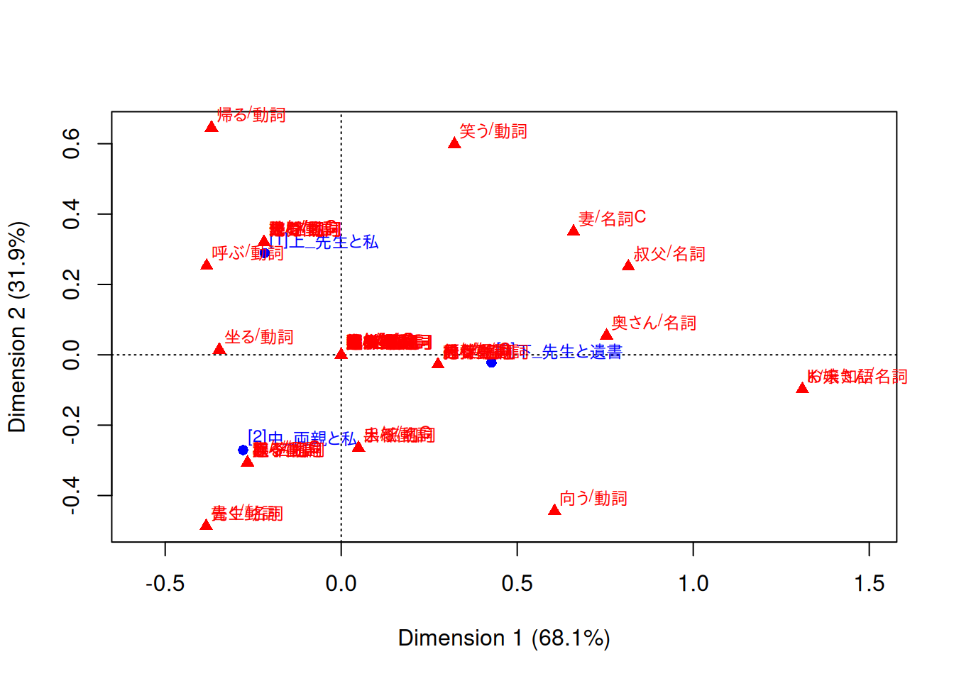
C.2.3 バイプロット(バブルプロット)
ggplot2でバイプロットを描画するには、たとえば次のようにします。ggrepel::geom_text_repel()でラベルを出す語彙の選択の仕方は、もうすこし工夫したほうがよいかもしれないです。
なお、このコードはCorrespondence Analysis visualization using ggplot | R-bloggersを参考にしました。
tf <- dfm |>
  tidytext::tidy() |>
  dplyr::left_join(
    dplyr::select(tbl, doc_id, section),
    by = dplyr::join_by(document == doc_id)
  ) |>
  dplyr::summarise(tf = sum(count), .by = term) |>
  dplyr::pull(tf, term)

# modified from https://www.r-bloggers.com/2019/08/correspondence-analysis-visualization-using-ggplot/
make_ca_plot_df <- function(ca.plot.obj, row.lab = "Rows", col.lab = "Columns") {
  tibble::tibble(
    Label = c(
      rownames(ca.plot.obj$rows),
      rownames(ca.plot.obj$cols)
    ),
    Dim1 = c(
      ca.plot.obj$rows[, 1],
      ca.plot.obj$cols[, 1]
    ),
    Dim2 = c(
      ca.plot.obj$rows[, 2],
      ca.plot.obj$cols[, 2]
    ),
    Variable = c(
      rep(row.lab, nrow(ca.plot.obj$rows)),
      rep(col.lab, nrow(ca.plot.obj$cols))
    )
  )
}
dat <- dat |>
  make_ca_plot_df(row.lab = "Construction", col.lab = "Medium") |>
  dplyr::mutate(
    Size = dplyr::if_else(Variable == "Construction", mean(tf), tf[Label])
  )
# 非ASCII文字のラベルに対してwarningを出さないようにする
suppressWarnings({
  ca_sum <- summary(ca_fit)
  dim_var_percs <- ca_sum$scree[, "values2"]
})

dat |>
  ggplot(aes(x = Dim1, y = Dim2, col = Variable, label = Label)) +
  geom_vline(xintercept = 0, lty = "dashed", alpha = .5) +
  geom_hline(yintercept = 0, lty = "dashed", alpha = .5) +
  geom_jitter(aes(size = Size), alpha = .3, show.legend = FALSE) +
  ggrepel::geom_label_repel(
    data = \(x) dplyr::filter(x, Variable == "Construction"),
    show.legend = FALSE
  ) +
  ggrepel::geom_text_repel(
    data = \(x) dplyr::filter(x, Variable == "Medium", sqrt(Dim1^2 + Dim2^2) > 0.25),
    show.legend = FALSE
  ) +
  scale_x_continuous(
    limits = range(dat$Dim1) +
      c(diff(range(dat$Dim1)) * -0.2, diff(range(dat$Dim1)) * 0.2)
  ) +
  scale_y_continuous(
    limits = range(dat$Dim2) +
      c(diff(range(dat$Dim2)) * -0.2, diff(range(dat$Dim2)) * 0.2)
  ) +
  scale_size_area(max_size = 16) +
  labs(
    x = paste0("Dimension 1 (", signif(dim_var_percs[1], 3), "%)"),
    y = paste0("Dimension 2 (", signif(dim_var_percs[2], 3), "%)")
  ) +
  theme_classic()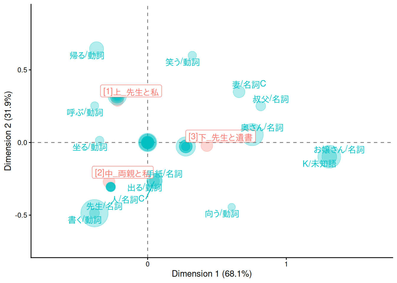
C.3 多次元尺度構成法(A.5.8)
C.3.1 MDS・バブルプロット
MASS::isoMDS()よりMASS::sammon()のほうがたぶん見やすいです。
simil <- dfm |>
  quanteda::dfm_weight(scheme = "boolean") |>
  proxyC::simil(margin = 2, method = "jaccard")

dat <- MASS::sammon(1 - simil, k = 2) |>
  purrr::pluck("points")
#> Initial stress        : 0.62279
#> stress after   0 iters: 0.62279
dat <- dat |>
dplyr::as_tibble(
rownames = "label",
.name_repair = ~ c("Dim1", "Dim2")
) |>
dplyr::mutate(
size = tf[label],
clust = (hclust(
proxyC::dist(dat, method = "euclidean") |> as.dist(),
method = "ward.D2"
) |> cutree(k = 6))[label]
)
dat |>
ggplot(aes(x = Dim1, y = Dim2, label = label, col = factor(clust))) +
geom_point(aes(size = size), alpha = .3, show.legend = FALSE) +
ggrepel::geom_text_repel(show.legend = FALSE) +
scale_size_area(max_size = 16) +
theme_classic()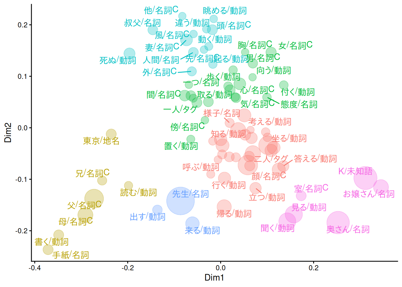
duckdb::dbDisconnect(con)
duckdb::duckdb_shutdown(drv)

sessioninfo::session_info(info = "packages")
#> ═ Session info ═══════════════════════════════════════════════════════════════
#> ─ Packages ───────────────────────────────────────────────────────────────────
#>  package      * version  date (UTC) lib source
#>  arules       * 1.7.13   2026-01-10 [1] RSPM (R 4.5.0)
#>  arulesViz    * 1.5.4    2025-08-21 [1] RSPM (R 4.5.0)
#>  audubon        0.6.2    2026-01-09 [1] RSPM (R 4.5.0)
#>  blob           1.3.0    2026-01-14 [1] RSPM (R 4.5.0)
#>  ca           * 0.71.1   2020-01-24 [1] RSPM (R 4.5.0)
#>  cachem         1.1.0    2024-05-16 [1] RSPM
#>  cellranger     1.1.0    2016-07-27 [1] RSPM (R 4.5.0)
#>  cli            3.6.5    2025-04-23 [1] RSPM
#>  codetools      0.2-20   2024-03-31 [2] CRAN (R 4.5.3)
#>  crosstalk      1.2.2    2025-08-26 [1] RSPM (R 4.5.0)
#>  curl           7.0.0    2025-08-19 [1] RSPM
#>  data.table     1.18.2.1 2026-01-27 [1] RSPM (R 4.5.0)
#>  DBI          * 1.3.0    2026-02-25 [1] RSPM (R 4.5.0)
#>  dbplyr         2.5.2    2026-02-13 [1] RSPM (R 4.5.0)
#>  digest         0.6.39   2025-11-19 [1] RSPM
#>  dplyr          1.2.0    2026-02-03 [1] RSPM (R 4.5.0)
#>  duckdb       * 1.5.0    2026-03-14 [1] RSPM (R 4.5.0)
#>  evaluate       1.0.5    2025-08-27 [1] RSPM
#>  farver         2.1.2    2024-05-13 [1] RSPM (R 4.5.0)
#>  fastmap        1.2.0    2024-05-15 [1] RSPM
#>  fastmatch      1.1-8    2026-01-17 [1] RSPM (R 4.5.0)
#>  foreach        1.5.2    2022-02-02 [1] RSPM (R 4.5.0)
#>  generics       0.1.4    2025-05-09 [1] RSPM (R 4.5.0)
#>  ggforce        0.5.0    2025-06-18 [1] RSPM (R 4.5.0)
#>  ggplot2      * 4.0.2    2026-02-03 [1] RSPM (R 4.5.0)
#>  ggraph         2.2.2    2025-08-24 [1] RSPM (R 4.5.0)
#>  ggrepel        0.9.8    2026-03-17 [1] RSPM (R 4.5.0)
#>  gibasa         1.1.3    2026-03-24 [1] Github (paithiov909/gibasa@4d450d2)
#>  glue           1.8.0    2024-09-30 [1] RSPM
#>  graphlayouts   1.2.3    2026-02-21 [1] RSPM (R 4.5.0)
#>  gridExtra      2.3      2017-09-09 [1] RSPM (R 4.5.0)
#>  gtable         0.3.6    2024-10-25 [1] RSPM (R 4.5.0)
#>  htmltools      0.5.9    2025-12-04 [1] RSPM
#>  htmlwidgets    1.6.4    2023-12-06 [1] RSPM
#>  httr           1.4.8    2026-02-13 [1] RSPM (R 4.5.0)
#>  igraph         2.2.2    2026-02-12 [1] RSPM
#>  iterators      1.0.14   2022-02-05 [1] RSPM (R 4.5.0)
#>  janeaustenr    1.0.0    2022-08-26 [1] RSPM (R 4.5.0)
#>  jsonlite       2.0.0    2025-03-27 [1] RSPM
#>  knitr          1.51     2025-12-20 [1] RSPM
#>  labeling       0.4.3    2023-08-29 [1] RSPM (R 4.5.0)
#>  lattice        0.22-9   2026-02-09 [2] CRAN (R 4.5.3)
#>  lazyeval       0.2.2    2019-03-15 [1] RSPM
#>  lifecycle      1.0.5    2026-01-08 [1] RSPM
#>  magrittr       2.0.4    2025-09-12 [1] RSPM
#>  MASS           7.3-65   2025-02-28 [2] CRAN (R 4.5.3)
#>  Matrix       * 1.7-4    2025-08-28 [2] CRAN (R 4.5.3)
#>  memoise        2.0.1    2021-11-26 [1] RSPM
#>  otel           0.2.0    2025-08-29 [1] RSPM
#>  pillar         1.11.1   2025-09-17 [1] RSPM
#>  pkgconfig      2.0.3    2019-09-22 [1] RSPM
#>  plotly         4.12.0   2026-01-24 [1] RSPM (R 4.5.0)
#>  polyclip       1.10-7   2024-07-23 [1] RSPM (R 4.5.0)
#>  proxyC         0.5.2    2025-04-25 [1] RSPM (R 4.5.0)
#>  purrr          1.2.1    2026-01-09 [1] RSPM
#>  quanteda       4.3.1    2025-07-10 [1] RSPM (R 4.5.0)
#>  R.cache        0.17.0   2025-05-02 [1] RSPM
#>  R.methodsS3    1.8.2    2022-06-13 [1] RSPM
#>  R.oo           1.27.1   2025-05-02 [1] RSPM
#>  R.utils        2.13.0   2025-02-24 [1] RSPM
#>  R6             2.6.1    2025-02-15 [1] RSPM
#>  RColorBrewer   1.1-3    2022-04-03 [1] RSPM (R 4.5.0)
#>  Rcpp           1.1.1    2026-01-10 [1] RSPM
#>  RcppParallel   5.1.11-2 2026-03-05 [1] RSPM (R 4.5.0)
#>  readxl         1.4.5    2025-03-07 [1] RSPM (R 4.5.0)
#>  registry       0.5-1    2019-03-05 [1] RSPM (R 4.5.0)
#>  rlang          1.1.7    2026-01-09 [1] RSPM
#>  rmarkdown      2.30     2025-09-28 [1] RSPM
#>  S7             0.2.1    2025-11-14 [1] RSPM (R 4.5.0)
#>  scales         1.4.0    2025-04-24 [1] RSPM (R 4.5.0)
#>  seriation      1.5.8    2025-08-20 [1] RSPM (R 4.5.0)
#>  sessioninfo    1.2.3    2025-02-05 [1] RSPM
#>  SnowballC      0.7.1    2023-04-25 [1] RSPM (R 4.5.0)
#>  stopwords      2.3      2021-10-28 [1] RSPM (R 4.5.0)
#>  stringi        1.8.7    2025-03-27 [1] RSPM
#>  stringr        1.6.0    2025-11-04 [1] RSPM
#>  styler         1.11.0   2025-10-13 [1] RSPM
#>  tibble         3.3.1    2026-01-11 [1] RSPM
#>  tidygraph      1.3.1    2024-01-30 [1] RSPM (R 4.5.0)
#>  tidyr          1.3.2    2025-12-19 [1] RSPM (R 4.5.0)
#>  tidyselect     1.2.1    2024-03-11 [1] RSPM (R 4.5.0)
#>  tidytext       0.4.3    2025-07-25 [1] RSPM (R 4.5.0)
#>  tokenizers     0.3.0    2022-12-22 [1] RSPM (R 4.5.0)
#>  TSP            1.2.7    2026-03-23 [1] RSPM (R 4.5.0)
#>  tweenr         2.0.3    2024-02-26 [1] RSPM (R 4.5.0)
#>  utf8           1.2.6    2025-06-08 [1] RSPM
#>  V8             8.0.1    2025-10-10 [1] RSPM (R 4.5.0)
#>  vctrs          0.7.2    2026-03-21 [1] RSPM (R 4.5.0)
#>  viridis        0.6.5    2024-01-29 [1] RSPM (R 4.5.0)
#>  viridisLite    0.4.3    2026-02-04 [1] RSPM (R 4.5.0)
#>  visNetwork     2.1.4    2025-09-04 [1] RSPM (R 4.5.0)
#>  withr          3.0.2    2024-10-28 [1] RSPM
#>  xfun           0.57     2026-03-20 [1] RSPM (R 4.5.0)
#>  yaml           2.3.12   2025-12-10 [1] RSPM
#>
#>  [1] /usr/local/lib/R/site-library
#>  [2] /usr/local/lib/R/library
#>  * ── Packages attached to the search path.
#>
#> ──────────────────────────────────────────────────────────────────────────────