suppressPackageStartupMessages({
  library(ggplot2)
  library(duckdb)
})
drv <- duckdb::duckdb()
con <- duckdb::dbConnect(drv, dbdir = "tutorial_jp/kokoro.duckdb", read_only = TRUE)

tbl <-
  readxl::read_xls("tutorial_jp/kokoro.xls",
    col_names = c("text", "section", "chapter", "label"),
    skip = 1
  ) |>
  dplyr::mutate(
    doc_id = factor(dplyr::row_number()),
    dplyr::across(where(is.character), ~ audubon::strj_normalize(.))
  ) |>
  dplyr::filter(!gibasa::is_blank(text)) |>
dplyr::relocate(doc_id, text, section, label, chapter)Appendix D — 抽出語メニュー3
D.1 階層的クラスター分析(A.5.9)
D.1.1 非類似度のヒートマップ🍳
Jaccard係数を指定して非類似度のヒートマップを描くと、そもそもパターンがほとんど見えませんでした……。
dfm <-
  dplyr::tbl(con, "tokens") |>
  dplyr::filter(
    pos %in% c(
      "名詞", # "名詞B", "名詞C",
      "地名", "人名", "組織名", "固有名詞",
      "動詞", "未知語", "タグ"
    )
  ) |>
  dplyr::mutate(
    token = dplyr::if_else(is.na(original), token, original),
    token = paste(token, pos, sep = "/")
  ) |>
  dplyr::count(doc_id, token) |>
  dplyr::collect() |>
  tidytext::cast_dfm(doc_id, token, n)

dat <- dfm |>
  quanteda::dfm_trim(min_termfreq = 30, termfreq_type = "rank") |>
  quanteda::dfm_weight(scheme = "boolean") |>
  proxyC::simil(margin = 2, method = "dice") |>
  rlang::as_function(~ 1 - .)()

factoextra::fviz_dist(as.dist(dat))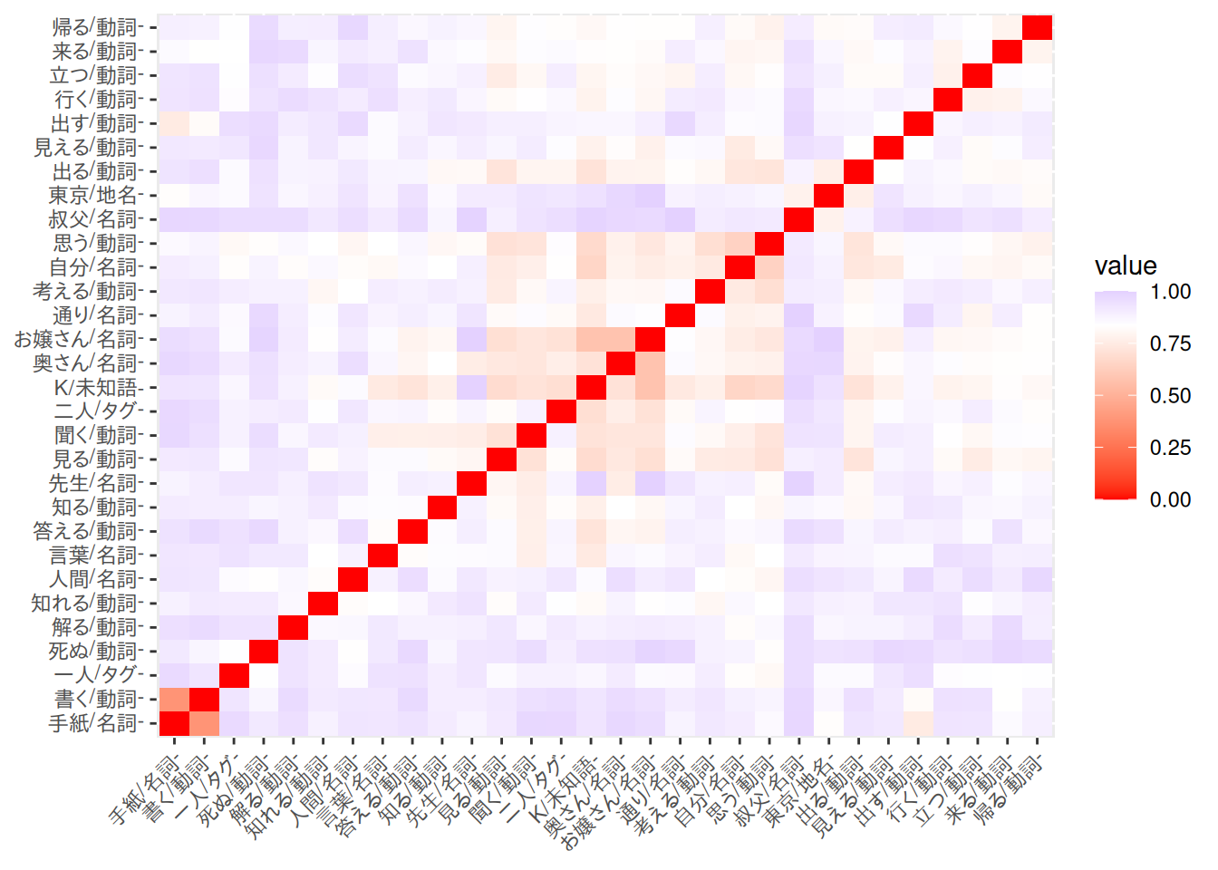
D.1.2 階層的クラスタリング
clusters <-
as.dist(dat) |>
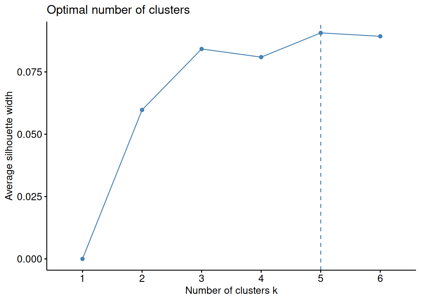
hclust(method = "ward.D2")D.1.3 シルエット分析🍳
factoextra::fviz_nbclust(
  as.matrix(dat),
  FUNcluster = factoextra::hcut,
  k.max = ceiling(sqrt(nrow(dat)))
)
cluster::silhouette(cutree(clusters, k = 5), dist = dat) |>
  factoextra::fviz_silhouette(print.summary = FALSE) +
  theme_classic()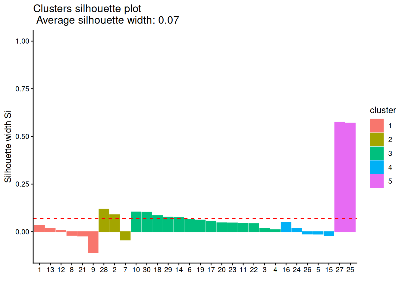
D.1.4 デンドログラム
デンドログラムについては、似たような表現を手軽に実現できる方法が見つけられません。ラベルの位置が左右反転していますが、factoextra::fviz_dend(horiz = TRUE)とするのが簡単かもしれないです。
factoextra::fviz_dend(clusters, k = 5, horiz = TRUE, labels_track_height = 0.3)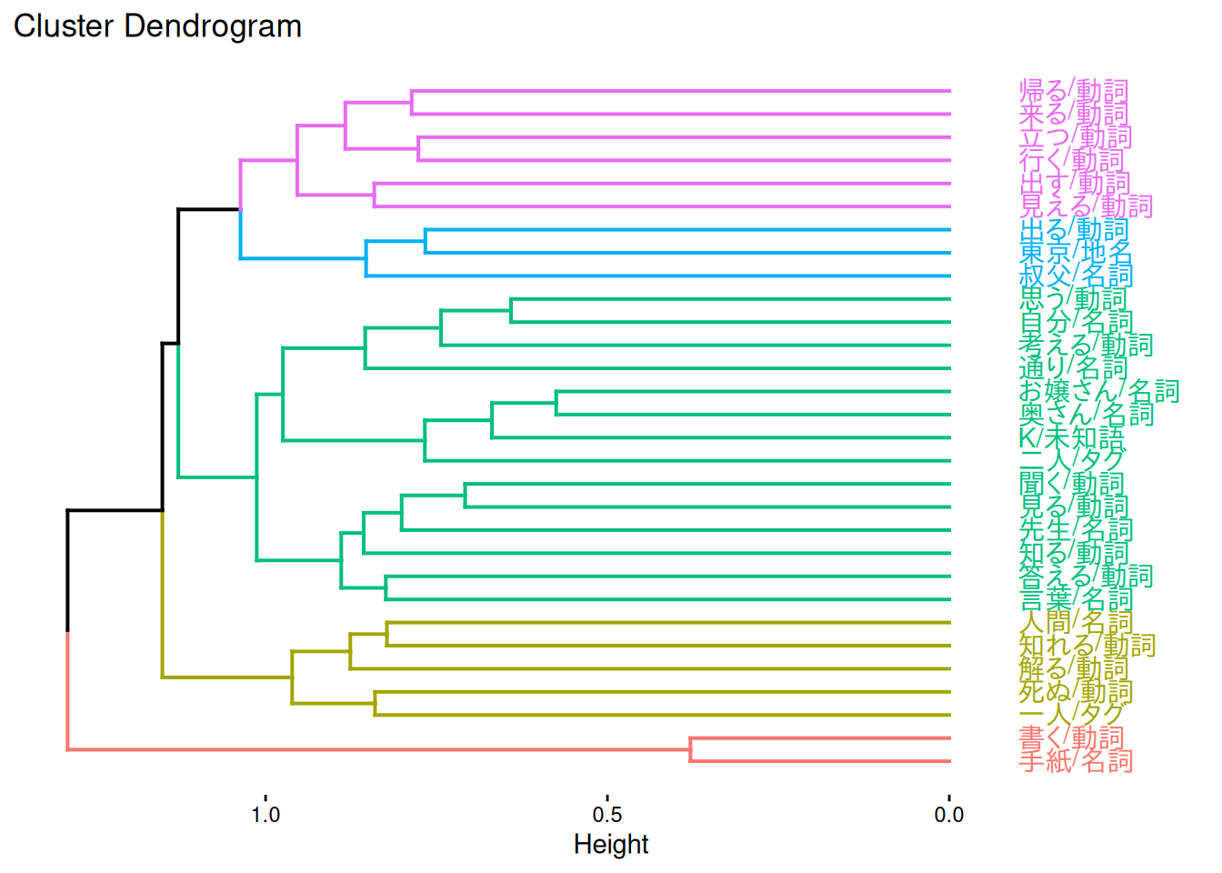
D.1.5 デンドログラムと棒グラフ
KH Coderのソースコードを見た感じ、デンドログラムと一緒に語の出現回数を描いている表現は、やや独特なことをしています。むしろ語の出現回数のほうが主な情報になってよいなら、ふつうの棒グラフの横にlegendry::scale_y_dendro()でデンドログラムを描くことができます。
dfm |>
  quanteda::dfm_trim(min_termfreq = 30, termfreq_type = "rank") |>
  quanteda::colSums() |>
  tibble::enframe() |>
  dplyr::mutate(
    clust = (clusters |> cutree(k = 5))[name]
  ) |>
  ggplot(aes(x = value, y = name, fill = factor(clust))) +
  geom_bar(stat = "identity", show.legend = FALSE) +
  scale_x_sqrt() +
  legendry::scale_y_dendro(clust = clusters) +
  labs(x = "出現回数", y = element_blank()) +
  theme_bw()
#> Warning: `label` cannot be a <ggplot2::element_blank> object.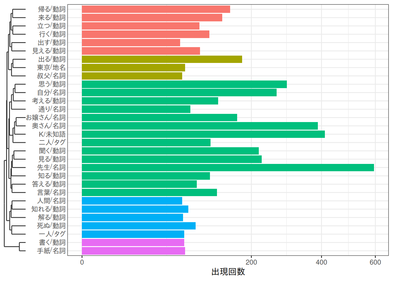
D.2 共起ネットワーク(A.5.10)
D.2.1 グラフの作成
描画するグラフをtbl_graphとして作成します。
dfm <-
  dplyr::tbl(con, "tokens") |>
  dplyr::filter(
    pos %in% c(
      "名詞", # "名詞B", "名詞C",
      "地名", "人名", "組織名", "固有名詞",
      "動詞", "未知語", "タグ"
    )
  ) |>
  dplyr::mutate(
    token = dplyr::if_else(is.na(original), token, original),
    token = paste(token, pos, sep = "/")
  ) |>
  dplyr::count(doc_id, token) |>
  dplyr::collect() |>
  tidytext::cast_dfm(doc_id, token, n)

dat <- dfm |>
  quanteda::dfm_trim(min_termfreq = 45, termfreq_type = "count") |>
  quanteda::dfm_weight(scheme = "boolean") |>
  proxyC::simil(margin = 2, method = "jaccard", rank = 3) |>
  as.matrix() |>
  tidygraph::as_tbl_graph(directed = FALSE) |>
  dplyr::distinct() |> # 重複を削除
  tidygraph::activate(edges) |>
  dplyr::filter(from != to)

dat
#> # A tbl_graph: 47 nodes and 82 edges
#> #
#> # An undirected simple graph with 2 components
#> #
#> # Edge Data: 82 × 3 (active)
#>     from    to weight
#>    <int> <int>  <dbl>
#>  1     1    11 0.137
#>  2     1    17 0.139
#>  3     2     4 0.120
#>  4     2    25 0.125
#>  5     3    10 0.0957
#>  6     3    25 0.106
#>  7     3    30 0.0909
#>  8     4    21 0.120
#>  9     5    44 0.171
#> 10     5    46 0.180
#> # ℹ 72 more rows
#> #
#> # Node Data: 47 × 1
#>   name
#>   <chr>
#> 1 先生/名詞
#> 2 帰る/動詞
#> 3 一人/タグ
#> # ℹ 44 more rows
D.2.2 相関係数の計算
ggraph::geom_edge_link2()のalphaに渡す相関係数を計算します。このあたりのコードは書くのが難しかったので、あまりスマートなやり方ではないかもしれません。
KH Coderには、それぞれの共起が文書集合内のどのあたりの位置に出現したかを概観できるようにするために、共起ネットワーク中のエッジについて、共起の出現位置との相関係数によって塗り分ける機能があります。これを実現するには、まずそれぞれの文書について文書集合内での通し番号を振ったうえで、それぞれの文書についてエッジとして描きたい共起の有無を1, 0で表してから、通し番号とのあいだの相関係数を計算します。
まず、共起ネットワーク中に描きこむ共起と、それらを含む文書番号をリストアップした縦長のデータフレームをつくります。
nodes <- tidygraph::activate(dat, nodes) |> dplyr::pull("name")
from <- nodes[tidygraph::activate(dat, edges) |> dplyr::pull("from")]
to <- nodes[tidygraph::activate(dat, edges) |> dplyr::pull("to")]

has_coocurrences <-
  dplyr::tbl(con, "tokens") |>
  dplyr::filter(
    pos %in% c(
      "名詞", # "名詞B", "名詞C",
      "地名", "人名", "組織名", "固有名詞",
      "動詞", "未知語", "タグ"
    )
  ) |>
  dplyr::mutate(
    token = dplyr::if_else(is.na(original), token, original),
    token = paste(token, pos, sep = "/")
  ) |>
  dplyr::filter(token %in% nodes) |>
  dplyr::collect() |>
  dplyr::reframe(
    from = from,
    to = to,
    has_from = purrr::map_lgl(from, ~ . %in% token),
    has_to = purrr::map_lgl(to, ~ . %in% token),
    .by = doc_id
  ) |>
  dplyr::filter(has_from & has_to) |>
  dplyr::group_by(from, to) |>
  dplyr::reframe(doc_id = doc_id)

has_coocurrences
#> # A tibble: 2,164 × 3
#>    from          to       doc_id
#>    <chr>         <chr>     <int>
#>  1 お嬢さん/名詞 K/未知語   1034
#>  2 お嬢さん/名詞 K/未知語   1035
#>  3 お嬢さん/名詞 K/未知語   1041
#>  4 お嬢さん/名詞 K/未知語   1042
#>  5 お嬢さん/名詞 K/未知語   1045
#>  6 お嬢さん/名詞 K/未知語   1046
#>  7 お嬢さん/名詞 K/未知語   1048
#>  8 お嬢さん/名詞 K/未知語   1049
#>  9 お嬢さん/名詞 K/未知語   1052
#> 10 お嬢さん/名詞 K/未知語   1054
#> # ℹ 2,154 more rows
次に、このデータフレームを共起ごとにグルーピングして、共起の有無と通し番号とのあいだの相関係数を含むデータフレームをつくります。
correlations <- has_coocurrences |>
  dplyr::group_by(from, to) |>
  dplyr::group_map(\(.x, .y) {
    tibble::tibble(
      doc_number = seq_len(nrow(tbl)),
      from = which(nodes == .y$from),
      to = which(nodes == .y$to)
    ) |>
      dplyr::group_by(from, to) |>
      dplyr::summarise(
        cor = cor(doc_number, as.numeric(doc_number %in% .x[["doc_id"]])),
        .groups = "drop"
      )
  }) |>
  purrr::list_rbind()

correlations
#> # A tibble: 82 × 3
#>     from    to     cor
#>    <int> <int>   <dbl>
#>  1    44    46  0.292
#>  2    44    45  0.139
#>  3     3    25  0.104
#>  4     3    30  0.0467
#>  5     3    10  0.145
#>  6     5    46  0.246
#>  7     5    44  0.199
#>  8    29    44  0.158
#>  9    29    36  0.104
#> 10     1    17 -0.176
#> # ℹ 72 more rows最後に、相関係数をtbl_graphのエッジと結合します。
dat <- dat |>
  tidygraph::activate(edges) |>
  dplyr::left_join(correlations, by = dplyr::join_by(from == from, to == to))
D.2.3 共起ネットワーク
上の処理が間違っていなければ、文書集合の後のほうによく出てくる共起であるほど、エッジの色が濃くなっているはずです。
dat |>
  tidygraph::activate(nodes) |>
  dplyr::mutate(
    community = factor(tidygraph::group_leading_eigen())
  ) |>
  ggraph::ggraph(layout = "fr") +
  ggraph::geom_edge_link2(
    aes(
      alpha = dplyr::percent_rank(cor) + .01, # パーセンタイルが0だと透明になってしまうので、適当に下駄をはかせる
      width = dplyr::percent_rank(weight) + 1
    ),
    colour = "red"
  ) +
  ggraph::geom_node_point(aes(colour = community), show.legend = FALSE) +
  ggraph::geom_node_label(aes(colour = community, label = name), repel = TRUE, show.legend = FALSE) +
  ggraph::theme_graph()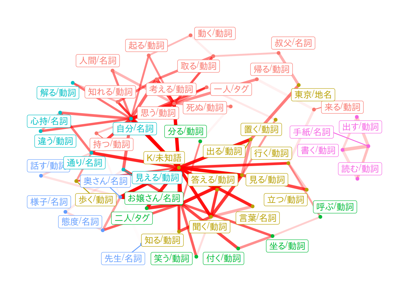
D.3 自己組織化マップ(A.5.11)
D.3.1 自己組織化マップ(SOM)
SOMの実装としては、KH Coderはsomを使っているようですが、kohonenを使ったほうがよいです。
行列が非常に大きい場合にはkohonen::som(mode = "online")としてもよいでしょうが、一般にバッチ型のほうが収束が早く、数十ステップ程度回せば十分とされます。
与える単語文書行列は、ここではtidytext::bind_tf_idf()を使ってTF-IDFで重みづけし、上位100語ほど抽出します。
dat <-
  dplyr::tbl(con, "tokens") |>
  dplyr::filter(
    pos %in% c(
      "名詞", # "名詞B", "名詞C",
      "地名", "人名", "組織名", "固有名詞",
      "動詞", "未知語", "タグ"
    )
  ) |>
  dplyr::mutate(
    token = dplyr::if_else(is.na(original), token, original),
    token = paste(token, pos, sep = "/")
  ) |>
  dplyr::count(doc_id, token) |>
  dplyr::collect() |>
  tidytext::bind_tf_idf(token, doc_id, n) |>
  tidytext::cast_dfm(doc_id, token, tf_idf) |>
  quanteda::dfm_trim(
    min_termfreq = 100,
    termfreq_type = "rank"
  ) |>
  as.matrix() |>
  scale() |>
  t()

som_fit <-
  kohonen::som(
    dat,
    grid = kohonen::somgrid(20, 16, "hexagonal"),
    rlen = 50, # 学習回数
    alpha = c(0.05, 0.01),
    radius = 8,
    dist.fcts = "sumofsquares",
    mode = "batch",
    init = aweSOM::somInit(dat, 20, 16)
)aweSOM::somQuality(som_fit, dat)
#>
#> ## Quality measures:
#> * Quantization error : 66.18159
#> * (% explained variance) : 94.1
#> * Topographic error : 0.38
#> * Kaski-Lagus error : 23.57054
#>
#> ## Number of obs. per map cell:
#> 1 2 3 4 5 6 7 8 9 10 11 12 13 14 15 16 17 18 19 20
#> 1 0 0 1 0 0 1 1 0 0 1 0 0 1 0 0 1 1 0 2
#> 21 22 23 24 25 26 27 28 29 30 31 32 33 34 35 36 37 38 39 40
#> 1 0 1 0 0 0 0 0 0 0 1 0 0 1 1 0 0 0 0 0
#> 41 42 43 44 45 46 47 48 49 50 51 52 53 54 55 56 57 58 59 60
#> 0 0 0 1 1 0 0 1 0 0 0 0 0 0 0 1 0 0 0 1
#> 61 62 63 64 65 66 67 68 69 70 71 72 73 74 75 76 77 78 79 80
#> 0 0 0 0 0 0 1 1 0 0 0 0 2 1 0 0 0 0 1 0
#> 81 82 83 84 85 86 87 88 89 90 91 92 93 94 95 96 97 98 99 100
#> 1 0 0 0 1 0 0 0 0 0 1 0 0 0 0 1 0 0 1 1
#> 101 102 103 104 105 106 107 108 109 110 111 112 113 114 115 116 117 118 119 120
#> 0 0 2 0 0 0 0 0 0 0 0 1 1 0 0 2 0 0 0 0
#> 121 122 123 124 125 126 127 128 129 130 131 132 133 134 135 136 137 138 139 140
#> 0 0 0 0 0 1 0 1 1 0 0 0 0 0 0 1 1 1 0 0
#> 141 142 143 144 145 146 147 148 149 150 151 152 153 154 155 156 157 158 159 160
#> 1 0 0 1 0 0 0 1 0 1 0 0 0 1 0 0 0 1 1 2
#> 161 162 163 164 165 166 167 168 169 170 171 172 173 174 175 176 177 178 179 180
#> 0 0 1 0 1 1 0 0 0 0 0 0 0 0 0 0 0 0 0 0
#> 181 182 183 184 185 186 187 188 189 190 191 192 193 194 195 196 197 198 199 200
#> 1 0 0 0 0 0 0 0 1 0 0 1 0 0 0 1 0 0 0 0
#> 201 202 203 204 205 206 207 208 209 210 211 212 213 214 215 216 217 218 219 220
#> 0 1 0 0 0 0 0 1 0 0 0 0 0 1 0 0 1 0 1 0
#> 221 222 223 224 225 226 227 228 229 230 231 232 233 234 235 236 237 238 239 240
#> 1 0 1 1 0 2 0 0 1 1 1 0 0 1 1 0 0 0 1 0
#> 241 242 243 244 245 246 247 248 249 250 251 252 253 254 255 256 257 258 259 260
#> 0 0 1 0 1 1 0 0 0 1 0 0 1 1 0 0 1 0 0 1
#> 261 262 263 264 265 266 267 268 269 270 271 272 273 274 275 276 277 278 279 280
#> 1 0 0 0 0 0 0 0 0 0 0 0 1 0 1 0 0 0 0 0
#> 281 282 283 284 285 286 287 288 289 290 291 292 293 294 295 296 297 298 299 300
#> 0 0 0 0 0 1 1 1 0 0 0 0 0 0 0 0 0 0 0 0
#> 301 302 303 304 305 306 307 308 309 310 311 312 313 314 315 316 317 318 319 320
#> 1 0 1 1 0 0 0 0 0 1 1 0 0 1 1 0 1 1 0 1D.3.2 U-Matrix
U-matrixは「各ノードの参照ベクトルが近傍ノードと異なる度合いで色づけする方法」(自己組織化マップ入門)です。暖色の箇所はデータ密度が低い「山間部」で、寒色の箇所はデータ密度が高い「平野部」みたいなイメージ、写像の勾配が急峻になっている箇所を境にしてクラスタが分かれていると判断するみたいな見方をします。
aweSOM::aweSOMsmoothdist(som_fit)
#> Warning: `aes_string()` was deprecated in ggplot2 3.0.0.
#> ℹ Please use tidy evaluation idioms with `aes()`.
#> ℹ See also `vignette("ggplot2-in-packages")` for more information.
#> ℹ The deprecated feature was likely used in the aweSOM package.
#>   Please report the issue to the authors.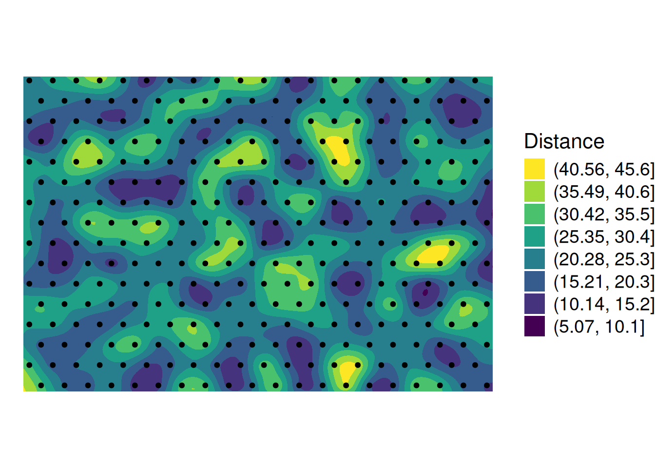
aweSOM::aweSOMplot(
  som_fit,
  data = dat,
  type = "UMatrix"
)
D.3.3 ヒットマップ🍳
色を付けるためのクラスタリングをしておきます。一部の「山間部」や「盆地」がクラスタになって、後はその他の部分みたいな感じに分かれるようですが、解釈するのに便利な感じで分かれてはくれなかったりします。
clusters <- som_fit |>
  purrr::pluck("codes", 1) |> # 参照ベクトル(codebook vectors)は`codes`にリストとして格納されている
  dist() |>
  hclust(method = "ward.D2") |>
  cutree(k = 10)
ヒットマップ(hitmap, proportion map)は以下のような可視化の方法です。ノードの中の六角形は各ノードが保持する参照ベクトルの数(比率)を表しています。ノードの背景色が上のコードで得たクラスタに対応します。
aweSOM::aweSOMplot(
  som_fit,
  data = dat,
  type = "Hitmap",
  superclass = clusters
)duckdb::dbDisconnect(con)
duckdb::duckdb_shutdown(drv)
sessioninfo::session_info(info = "packages")
#> ═ Session info ═══════════════════════════════════════════════════════════════
#> ─ Packages ───────────────────────────────────────────────────────────────────
#> package * version date (UTC) lib source
#> abind 1.4-8 2024-09-12 [1] RSPM (R 4.5.0)
#> audubon 0.6.2 2026-01-09 [1] RSPM (R 4.5.0)
#> aweSOM 1.3 2022-08-30 [1] RSPM (R 4.5.0)
#> backports 1.5.0 2024-05-23 [1] RSPM
#> blob 1.3.0 2026-01-14 [1] RSPM (R 4.5.0)
#> broom 1.0.12 2026-01-27 [1] RSPM (R 4.5.0)
#> car 3.1-5 2026-02-03 [1] RSPM (R 4.5.0)
#> carData 3.0-6 2026-01-30 [1] RSPM (R 4.5.0)
#> cellranger 1.1.0 2016-07-27 [1] RSPM (R 4.5.0)
#> class 7.3-23 2025-01-01 [2] CRAN (R 4.5.3)
#> cli 3.6.5 2025-04-23 [1] RSPM
#> cluster 2.1.8.2 2026-02-05 [2] CRAN (R 4.5.3)
#> curl 7.0.0 2025-08-19 [1] RSPM
#> DBI * 1.3.0 2026-02-25 [1] RSPM (R 4.5.0)
#> dbplyr 2.5.2 2026-02-13 [1] RSPM (R 4.5.0)
#> dendextend 1.19.1 2025-07-15 [1] RSPM (R 4.5.0)
#> digest 0.6.39 2025-11-19 [1] RSPM
#> dotCall64 1.2 2024-10-04 [1] RSPM (R 4.5.0)
#> dplyr 1.2.0 2026-02-03 [1] RSPM (R 4.5.0)
#> duckdb * 1.5.0 2026-03-14 [1] RSPM (R 4.5.0)
#> e1071 1.7-17 2025-12-18 [1] RSPM (R 4.5.0)
#> evaluate 1.0.5 2025-08-27 [1] RSPM
#> factoextra 2.0.0 2026-03-03 [1] RSPM (R 4.5.0)
#> farver 2.1.2 2024-05-13 [1] RSPM (R 4.5.0)
#> fastmap 1.2.0 2024-05-15 [1] RSPM
#> fastmatch 1.1-8 2026-01-17 [1] RSPM (R 4.5.0)
#> fields 17.1 2025-09-08 [1] RSPM (R 4.5.0)
#> Formula 1.2-5 2023-02-24 [1] RSPM (R 4.5.0)
#> generics 0.1.4 2025-05-09 [1] RSPM (R 4.5.0)
#> ggplot2 * 4.0.2 2026-02-03 [1] RSPM (R 4.5.0)
#> ggpubr 0.6.3 2026-02-24 [1] RSPM (R 4.5.0)
#> ggrepel 0.9.8 2026-03-17 [1] RSPM (R 4.5.0)
#> ggsignif 0.6.4 2022-10-13 [1] RSPM (R 4.5.0)
#> gibasa 1.1.3 2026-03-24 [1] Github (paithiov909/gibasa@4d450d2)
#> glue 1.8.0 2024-09-30 [1] RSPM
#> gridExtra 2.3 2017-09-09 [1] RSPM (R 4.5.0)
#> gtable 0.3.6 2024-10-25 [1] RSPM (R 4.5.0)
#> htmltools 0.5.9 2025-12-04 [1] RSPM
#> htmlwidgets 1.6.4 2023-12-06 [1] RSPM
#> httpuv 1.6.17 2026-03-18 [1] RSPM (R 4.5.0)
#> igraph 2.2.2 2026-02-12 [1] RSPM
#> isoband 0.3.0 2025-12-07 [1] RSPM (R 4.5.0)
#> janeaustenr 1.0.0 2022-08-26 [1] RSPM (R 4.5.0)
#> jsonlite 2.0.0 2025-03-27 [1] RSPM
#> knitr 1.51 2025-12-20 [1] RSPM
#> kohonen 3.0.13 2026-01-22 [1] RSPM (R 4.5.0)
#> labeling 0.4.3 2023-08-29 [1] RSPM (R 4.5.0)
#> later 1.4.8 2026-03-05 [1] RSPM
#> lattice 0.22-9 2026-02-09 [2] CRAN (R 4.5.3)
#> legendry 0.2.4 2025-09-14 [1] RSPM (R 4.5.0)
#> lifecycle 1.0.5 2026-01-08 [1] RSPM
#> magrittr 2.0.4 2025-09-12 [1] RSPM
#> maps 3.4.3 2025-05-26 [1] RSPM (R 4.5.0)
#> Matrix 1.7-4 2025-08-28 [2] CRAN (R 4.5.3)
#> mime 0.13 2025-03-17 [1] RSPM
#> otel 0.2.0 2025-08-29 [1] RSPM
#> pillar 1.11.1 2025-09-17 [1] RSPM
#> pkgconfig 2.0.3 2019-09-22 [1] RSPM
#> promises 1.5.0 2025-11-01 [1] RSPM
#> proxy 0.4-29 2025-12-29 [1] RSPM (R 4.5.0)
#> proxyC 0.5.2 2025-04-25 [1] RSPM (R 4.5.0)
#> purrr 1.2.1 2026-01-09 [1] RSPM
#> quanteda 4.3.1 2025-07-10 [1] RSPM (R 4.5.0)
#> R.cache 0.17.0 2025-05-02 [1] RSPM
#> R.methodsS3 1.8.2 2022-06-13 [1] RSPM
#> R.oo 1.27.1 2025-05-02 [1] RSPM
#> R.utils 2.13.0 2025-02-24 [1] RSPM
#> R6 2.6.1 2025-02-15 [1] RSPM
#> RColorBrewer 1.1-3 2022-04-03 [1] RSPM (R 4.5.0)
#> Rcpp 1.1.1 2026-01-10 [1] RSPM
#> RcppParallel 5.1.11-2 2026-03-05 [1] RSPM (R 4.5.0)
#> readxl 1.4.5 2025-03-07 [1] RSPM (R 4.5.0)
#> rlang 1.1.7 2026-01-09 [1] RSPM
#> rmarkdown 2.30 2025-09-28 [1] RSPM
#> rstatix 0.7.3 2025-10-18 [1] RSPM (R 4.5.0)
#> S7 0.2.1 2025-11-14 [1] RSPM (R 4.5.0)
#> scales 1.4.0 2025-04-24 [1] RSPM (R 4.5.0)
#> sessioninfo 1.2.3 2025-02-05 [1] RSPM
#> shiny 1.13.0 2026-02-20 [1] RSPM
#> SnowballC 0.7.1 2023-04-25 [1] RSPM (R 4.5.0)
#> spam 2.11-3 2026-01-08 [1] RSPM (R 4.5.0)
#> stopwords 2.3 2021-10-28 [1] RSPM (R 4.5.0)
#> stringi 1.8.7 2025-03-27 [1] RSPM
#> styler 1.11.0 2025-10-13 [1] RSPM
#> tibble 3.3.1 2026-01-11 [1] RSPM
#> tidygraph 1.3.1 2024-01-30 [1] RSPM (R 4.5.0)
#> tidyr 1.3.2 2025-12-19 [1] RSPM (R 4.5.0)
#> tidyselect 1.2.1 2024-03-11 [1] RSPM (R 4.5.0)
#> tidytext 0.4.3 2025-07-25 [1] RSPM (R 4.5.0)
#> tokenizers 0.3.0 2022-12-22 [1] RSPM (R 4.5.0)
#> utf8 1.2.6 2025-06-08 [1] RSPM
#> V8 8.0.1 2025-10-10 [1] RSPM (R 4.5.0)
#> vctrs 0.7.2 2026-03-21 [1] RSPM (R 4.5.0)
#> viridis 0.6.5 2024-01-29 [1] RSPM (R 4.5.0)
#> viridisLite 0.4.3 2026-02-04 [1] RSPM (R 4.5.0)
#> withr 3.0.2 2024-10-28 [1] RSPM
#> xfun 0.57 2026-03-20 [1] RSPM (R 4.5.0)
#> xtable 1.8-8 2026-02-22 [1] RSPM
#> yaml 2.3.12 2025-12-10 [1] RSPM
#>
#> [1] /usr/local/lib/R/site-library
#> [2] /usr/local/lib/R/library
#> * ── Packages attached to the search path.
#>
#> ──────────────────────────────────────────────────────────────────────────────